Four Ways to Grow a Classifier, and Why the Safest One Cannot Learn
arXiv has just published a paper of mine: Four Ways to Grow a Classifier and Why One of Them Cannot Learn, arXiv:2610.00180. What follows is the paper in order, with the numbers, and the account of how it came to exist, because that part explains its shape.
It was not designed as a study. While building neural-trees, a scikit-learn compatible library of tree models that train by gradient descent, I had to settle four implementation questions about models that grow while they train. For each I wrote down the sensible-sounding option, implemented it, and measured it against the thing it was meant to improve on, under one fixed protocol. Three of the four traded one quantity for another. The fourth could not learn at all, and that one had a cause that could be proved rather than read off a table.
A small example says what these models are. A credit officer with one rule, "refuse if the loan runs longer than 24 months", is a decision tree of depth one. A soft version of the same officer does not refuse a 25-month loan outright: it sends most of that applicant down the refuse branch and a little down the accept branch, and the share depends on how far past 24 months the loan is. Because that share is a smooth function of the number, the rule can be trained by gradient descent, the way a neural network is. Growing is what happens when the officer, having stopped improving with one rule, adds a second question under one of the answers: "and if refused, does the applicant have savings?" The four decisions in the paper are four ways of adding that second question.
The numbers below are the paper's. In the repository, the measurement scripts under paper/arxiv/olcum write their results to JSON files, and doldur.py fills the placeholders in the manuscript template from those files, so the tables in the paper cannot drift from the code that produced them. The protocol is the same throughout: features standardised with training-fold statistics only, stratified five-fold cross-validation repeated with three seeds, fifteen fits per arm, the same folds and seeds for every arm. The standard deviations describe the spread across those fifteen fits and are not confidence intervals; where a yes or no was needed, the paper uses the combined 5x2cv F test.
Step 1. What "grow" means here
Keep the credit officer in mind. An ordinary decision tree works like that officer: one question at each node, yes or no, and every applicant takes exactly one path. A soft decision tree asks the same question but answers with a share. To "is the term longer than 24 months", a 25-month applicant passes eighty percent yes and twenty percent no; a 60-month applicant goes almost entirely to the yes side. The share is a smooth curve of how far the term sits from the threshold, a sigmoid. At the bottom of the tree every leaf holds a verdict, say "seventy percent good, thirty percent bad", and an applicant's result is the mixture of every leaf they reached, weighted by how much of them reached it.
The consequence is this. Because every question and every leaf is made of smooth numbers, the whole tree can be trained like a neural network, by gradient descent. And a tree that trains that way can be grown while it trains: add a question, keep training, the new question learns too. That is what "grow" means in the paper: adding structure to a model while training is under way.
There are four ways to add it, and the paper measures all four:
- Add a whole level at once. Put a new question under every leaf of the tree at the same time, arranged so that the tree's answers do not change at that moment. This is the one the story is about.
- Prepare a new neuron before adding it. This one is about a growing neural network rather than a tree. When the network stalls it adds a hidden unit; the question is whether to install that unit at random or to fit it to the network's current mistakes first.
- Split a single leaf. Instead of a level, put a question under one leaf at a time, the leaf where the most error has collected. It promises much smaller trees.
- Choose the kind of question. A node's question can look at one feature ("is the term longer than 24 months"), at a weighted sum of several, or draw a curved boundary. Taking the more powerful question only when it brings a measurable improvement sounds like the frugal choice.
All four are reasonable. Three give something and take something; one learns nothing at all.
Step 2. The operation everyone writes first
There is an obvious way to deepen a trained soft tree without losing anything it has learned. Take every leaf, turn it into a gate with all-zero weights, so that it sends exactly half of the mass each way, and give both new children the parent's distribution. Half of Q plus half of Q is Q, so the deeper tree computes precisely the function the shallower one did. Training continues from there and the extra capacity is available. It is the tree version of Net2Net, the 2016 recipe for making a trained neural network wider or deeper without changing its outputs so that training can continue instead of restarting, and of the network morphisms that generalised it; and it is the construction I wrote down first.
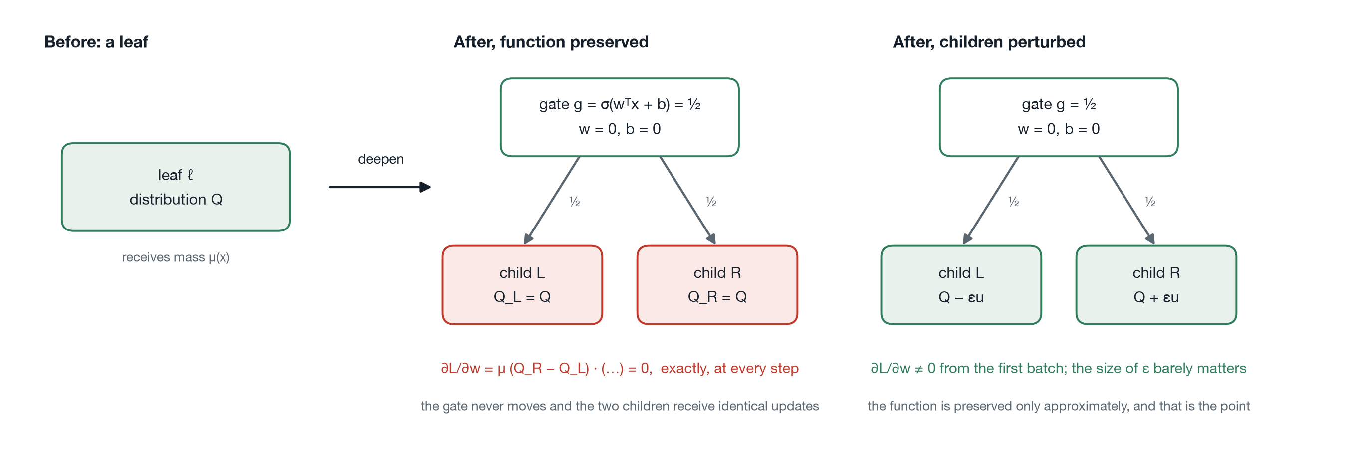
The new level never learned anything. Not slowly; never. The reason is a few lines of calculus. The subtree's contribution to the output is the mass arriving at the old leaf times a mixture of the two children, g times the right child plus (1 minus g) times the left. Differentiate with respect to the gate value g and you get the arriving mass times the difference between the two children. When the children are identical, that difference is the zero vector. The gate's weights and bias reach the loss only through g, so by the chain rule their gradient is exactly zero, whatever g is and whatever the loss is. That is the first half of the proposition. The second half: with the gate at one half, the two children receive identical gradients, so they stay identical. Put the two halves together and run induction over the training steps. At every step the gate gets no update and the children get the same update, so the condition that made the gradient zero is restored exactly, and the argument repeats forever.
I want to be precise about what does not rescue it. Momentum, Adam, weight decay: each of them rescales or accumulates a gradient that is zero, and weight decay shrinks two equal children by equal amounts. Mini-batches do not help, because both children see the same batch. And I checked, rather than assumed, that floating point noise does not break the tie: on a depth-two tree trained on Iris and then deepened, the sum of absolute gradients over every new gate is 0 in single precision, not small, and the sibling leaves' gradients are bitwise identical. That check runs in the library's continuous integration.
The contrast with the neural network literature is the point of the paper. Net2Net duplicates a unit, notes that the copies are symmetric, and adds noise. Splitting steepest descent shows a duplicated neuron sits at a saddle and derives the second-order direction out of it. GradMax zeroes the new weights but gives the unit a bias so the outgoing weights have something to follow. In all three the first-order information is weak but recoverable. In the tree gate case it is absent: the derivative is zero and it reproduces itself.
Step 3. What it costs, and where the cost comes from
The fix is to perturb the two children at insertion, in opposite directions, by a small random amount. The function is then preserved only approximately, which turns out to be the whole point.
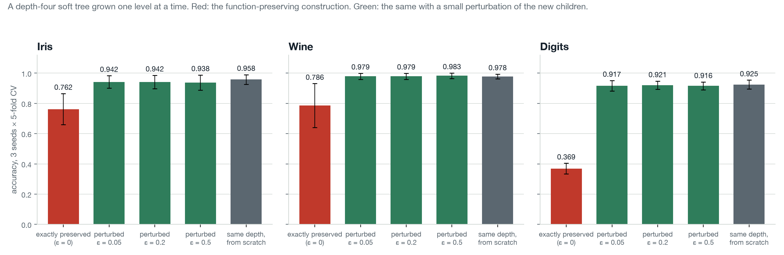
Exact preservation costs 19.6 accuracy points on Iris, 19.1 on Wine and 55.6 on Digits against the same depth trained from scratch. Between a perturbation of 0.05 and one of 0.5, a factor of ten, the means move by at most 0.4 points. The F test comparing zero against 0.2 gives p = 0.048 on Iris, 0.010 on Wine and below 0.0001 on Digits; the Iris value sits on the conventional line and I do not lean on it in the paper, because the test is conservative and the value crossed 0.05 when I moved the scaler inside the test's folds.
Those three datasets say the failure is real. They do not say when it is expensive, and the proposition does. A tree deepened this way computes the function of the tree it started from, which has two leaves. Two leaves can hold two distributions. On a two-class problem that is all the tree needs, so the dead levels should cost nothing; on a problem with K classes the tree can never reach the K leaves it needs, and the cost should grow with the number of classes and not with the number of features. The version on arXiv today reports the three datasets. The replacement I am submitting this week tests the prediction on twenty more from OpenML, and it holds: over 13 two-class datasets the mean cost is minus 0.2 points, which is to say none, and over 7 multi-class datasets it is 40.2 points, from 20 to 58, with the F test rejecting equality on every one. The Spearman correlation of the cost with the number of classes is 0.64; with the number of features, 0.03. The first draft said the failure costs "about twenty points". The right statement is that it costs whatever the gap is between the starting tree's capacity and the problem's need, which is zero or catastrophic and rarely in between.
Step 4. Does it matter how the symmetry is broken?
Random noise breaks the tie in an arbitrary direction, and a better direction seems available: the residual of the loss with respect to the leaf's distribution says which classes the leaf under-predicts, so the two children can be placed on either side of the parent along that direction, and the new gate can be pointed at the samples pulling one way. This is GradMax's idea applied to a tree gate. I implemented it, I expected it to help, and over 24 datasets it changes accuracy by +0.20 points on average against plain noise, median zero, with two F tests under 0.05 out of 24, which is what chance produces. The one measurable effect is stability: the fold-to-fold standard deviation on the multi-class datasets falls from 0.025 to 0.021. Once the gradient is nonzero, gradient descent finds the split on its own. The only thing the proposition asks of an initialisation is that the gradient not be zero.
Step 5. Where to put a new hidden unit
The second decision concerns a different model, Alpaydin's grow-and-learn network, which adds a hidden unit when training error stops improving. The original installs the unit with random weights, and a random unit perturbs every output the moment it arrives, damaging a network that was just judged to have stalled. The alternative follows cascade-correlation: freeze the network, compute its residual, train the candidate's incoming weights to correlate with that residual, and install it with zero outgoing weights. The function is unchanged at insertion, and this time that is safe, because the outgoing weights have a nonzero gradient as soon as the incoming ones carry any signal.
What it buys is a smaller network, on every dataset: Iris goes from 17.2 hidden units to 6.9, Wine from 6.3 to 4.3, Digits from 7.5 to 5.7. The mechanism is visible in the growth trace. A random unit arrives unhelpful, the error does not fall, the growth criterion fires again, and the network grows because growth is not working. Fitting the unit first removes that loop. What it does not buy is accuracy. Iris rose and Wine was identical, neither significantly, and on Digits accuracy fell by 2.1 points, which the F test does call significant, in favour of random initialisation. The likely reason is in the same table: the residual variant stops at 5.7 units where the random one keeps going to 7.5, and on a ten-class problem those units are doing work. Growth that stops early is parsimony on an easy problem and underfitting on a harder one, and the criterion cannot tell them apart. An earlier draft reported the Iris gain on its own. That is the kind of claim that survives exactly until somebody runs a fourth dataset.
One detail cost me a day and is in the paper so that it costs nobody else one. The candidate objective divides by the square root of a variance that can be zero on a degenerate batch. At zero the derivative of the square root is infinite and the whole network becomes NaN in one step. Clamping the variance before the root fixes it; clamping the result afterwards does not, because by then the gradient has already been formed.
Step 6. Which leaf to split
Instead of a whole level, a tree can grow one leaf at a time, splitting the leaf that carries the most expected error. That rule produces by far the sparsest trees, and on the twenty OpenML datasets it lost to a complete depth-six tree on 11, tied on 3 and won on 6, by 1.8 points on average, and it lost on every multi-class dataset. The sparsity was real, from 63 splits to somewhere between one and eighteen, and it looked as if it were paid for in accuracy.
It was paid for in a defect, and it was the same defect. When a leaf was split, the code marked the node as split and did nothing else: the children kept the untrained logits they were constructed with, so the split replaced the parent's learned distribution with a uniform one and started the children identical. Proposition at a single node instead of a whole level. The level-wise path had been cured of this; the per-leaf path had not. With the children inheriting the parent and the symmetry broken, per-leaf growth went from 8.3 points below the complete tree to 2.3 points below it, on average over eight multi-class datasets, using 23% of the splits. The direction of the symmetry breaking was, again, second-order; inheriting the parent is what changed the result.
Two other things separate a grown tree from one trained from scratch, and neither is growth. The grown tree holds out 10% of its training fold to decide whether the last step earned its place, and it divides its epoch budget across growth rounds. Measured separately, the holdout alone costs a fixed tree 0.4 points, and giving every growth round the full budget is worth 0.8 points over splitting it. Some of what looked like a cost of growing was a cost of having 10% less data, which is a different thing and should be stated as one.
Step 7. Choosing the split type at a node
The omnivariate tree picks each node's split type, a single-feature threshold, a linear split or a nonlinear one, by cross-validated accuracy on that node's data. That takes a nonlinear split over a simpler one for any improvement at all. Requiring the improvement to be significant, by the same F test, and otherwise keeping the simpler split, sounds strictly better. It is not. On Breast Cancer the tree gets larger, 4.7 nodes to 7.0, and less accurate, 0.971 to 0.958; on Digits larger for the same accuracy. A simpler split separates its node's data less cleanly, so the children inherit harder problems and have to be split in turn. Parsimony enforced locally is paid for globally. There is a structural problem too: the test needs a minimum sample count, and nodes get smaller with depth, so the criterion is least available exactly where a recursive method does most of its work. The option ships switched off.
What the four have in common
They line up on one axis: whether the optimiser has something to act on at the moment the new structure arrives. A unit fitted to the residual and installed with zero outgoing weights has a nonzero gradient immediately, and it reliably gives a smaller network. A leaf split into two children that inherit the parent and differ from each other has a nonzero gradient immediately, and it now comes within a few points of a complete tree at a fraction of the splits. A level of gates with identical children, or a leaf split into identical untrained children, leaves the optimiser nothing, and the cost is exactly the capacity the tree can no longer reach.
The axis predicts which operations can work. It does not predict how much they help, and steps 5 and 6 show that depends on the problem. Nor does it care how the symmetry is broken. The practical rule that falls out is narrow and cheap: when you add parameters to a differentiable model during training, compute their gradient on the first batch after insertion and assert that it is not zero. One line in a test. In this library it would have caught both defects.
What the paper does not claim
The datasets are of moderate size, at most 5 000 rows and 72 features after subsampling, and conclusions about accuracy should not be read as generalising beyond that. Each comparison is between arms of one implementation with settings held fixed; that isolates the operation under test and does not establish that the winning arm is the best available method, and step 6 is the reminder that an implementation detail of mine can be responsible for all of an effect. The proposition is exact and implementation-independent. Nothing else in the paper is. A second-order splitting direction in the manner of splitting steepest descent is the natural way to repair the operation without noise, and I have not tried it.
Where everything is
- Paper: arxiv.org/abs/2610.00180 (PDF)
- Code, the measurement script and the zero-gradient regression test: github.com/cgrtml/neural-trees
- The exact version measured, archived: doi.org/10.5281/zenodo.22929121 (v0.7.0)
- Install:
pip install neural-trees, pypi.org/project/neural-trees - Documentation, with the design decisions and their tables: cagritemel.com/neural-trees
- Try the models in the browser: neural-trees.streamlit.app
- What the library is for, with a credit-scoring case study: the previous post
If you train models that grow, run the one-line check. If it fails on your code, I would like to hear about it, and if it passes, I would like to hear that too.